WITSML import via Pandas and Python
In the last weeks example we took a look at connecting to Azure storage via python in order to directly import the files / data from the Volve dataset. As part of that analysis we looked at the types of file formats and saw that among many different types, xml was by far the most prevalent. Part of the '4 V's' of Data Science (volume, Variety, Velocity and Veracity) is variety. In the Volve dataset - last weeks analysis clearly showcased that variety (different types of data) is most certainly true in the oil and gas community. XML is a markup document that is prevalant outside of oil and gas. Within the petroleum industry xml files are typically WITSML files, which are xml files that follow a set of standards maintained by Energistics.
Energistics maintains an SDK for use in reading/developing/publishing WITSML files. These files can contain a large variety of data within themselves, common examples are: - Well logs such as those run with wireline tools - BHA or bottom hole assembly - containing information about the components that make up the bottom hole assembly (bit, motor, MWD, etc) - Survey information that defines the trajectory of the borehole
This SDK is written in C# programming language. There is also a package written in Java and developed by Hashmap. These packages work well - however C# and Java are not commonly used in the data science community. One future development in this blog is to develop and release a methodology in order to interact with WITSML files using Python contained in a package or library. For now however we will use this blog post in order to look at two different types of WISTML files (logs and trajectory) - the structure of these files and how to automatically parse them into pandas dataframes for use in data science routines, and optionally big data techniques such as spark and/or databases.
# Import required libraries & packages
from azure.storage.blob import BlockBlobService
import pandas as pd
import xml.etree.ElementTree as ET
from bs4 import BeautifulSoup
from collections import defaultdict
import seaborn as sns
import numpy as np
import matplotlib.pyplot as plt
%matplotlib inline
Connect to the Blob Storage from Last Week
# List the account name and sas_token *** I have removed the SAS token in order to allow the user to register properly thorugh Equinor's data portal
azure_storage_account_name = 'dataplatformblvolve'
sas_token = '###'

# Create a service and use the SAS
sas_blob_service = BlockBlobService(
    account_name=azure_storage_account_name,
    sas_token=sas_token,
)

filename = 'WITSML Realtime drilling data/Norway-StatoilHydro-15_$47$_9-F-14/1/log/1/1/1'

blob = sas_blob_service.list_blobs('pub', filename)
for b in blob:
    print(b.name)
WITSML Realtime drilling data/Norway-StatoilHydro-15_$47$_9-F-14/1/log/1/1/1/00001.xml
WITSML Realtime drilling data/Norway-StatoilHydro-15_$47$_9-F-14/1/log/1/1/1/00002.xml
WITSML Realtime drilling data/Norway-StatoilHydro-15_$47$_9-F-14/1/log/1/1/1/00003.xml
Above we have connected to a folder within the well 9-F-14 containing three different WITSML files of well logs. Below we will look at the structure of one of these files:
WITSML_file = 'WITSML Realtime drilling data/Norway-StatoilHydro-15_$47$_9-F-14/1/log/1/1/1/00001.xml'
blob = sas_blob_service.get_blob_to_text('pub', WITSML_file)
blob.content[:1000]
'<?xml version="1.0" encoding="UTF-8"?><logs xmlns="http://www.witsml.org/schemas/1series" xmlns:xsi="http://www.w3.org/2001/XMLSchema-instance" version="1.4.1.1"><log uidWell="W-353085" uidWellbore="B-353085" uid="L-567705-MD"><nameWell>15/9-F-14</nameWell><nameWellbore>15/9-F-14 - Main Wellbore</nameWellbore><name>MWD Geocervices Real Time Data 26in - MD Log</name><serviceCompany>Schlumberger</serviceCompany><runNumber>2</runNumber><pass>Drilling</pass><creationDate>2007-12-03T17:51:24.000Z</creationDate><indexType>measured depth</indexType><startIndex uom="m">0</startIndex><endIndex uom="m">457.011</endIndex><direction>increasing</direction><indexCurve>DEPTH</indexCurve><priv_dTimPriority>2007-12-03T17:51:24.000Z</priv_dTimPriority><logCurveInfo uid="G_IC5"><mnemonic>G_IC5</mnemonic><unit>ppm</unit><minIndex uom="m">193.999</minIndex><maxIndex uom="m">456.999</maxIndex><curveDescription>Gas, Iso-C5</curveDescription><dataSource>MudLog</dataSource><typeLogData>double</typeLogData></lo'
We can see by printing the first 1000 characters of the WITSML file that we do have XML tags that are associated to different information contained in the log file. It can be hard to interpret the xml file without parsing to better understand its organization and content. We will use beautiful soup which is a parsing library developed for xml and html in python. We can use it to read in our WITSML file and begin to make sense of it.
Explore WITSML file Structure
import glob, os
from bs4 import BeautifulSoup
master_df = pd.DataFrame()
soup = BeautifulSoup(blob.content, 'xml')
set([str(tag.name) for tag in soup.find_all()])
{'commonData',
 'creationDate',
 'curveDescription',
 'dTimCreation',
 'dTimLastChange',
 'data',
 'dataSource',
 'direction',
 'endIndex',
 'indexCurve',
 'indexType',
 'log',
 'logCurveInfo',
 'logData',
 'logs',
 'maxIndex',
 'minIndex',
 'mnemonic',
 'mnemonicList',
 'name',
 'nameWell',
 'nameWellbore',
 'pass',
 'priv_dTimPriority',
 'priv_dTimReceived',
 'priv_ipLastChange',
 'priv_ipOwner',
 'priv_userLastChange',
 'priv_userOwner',
 'runNumber',
 'serviceCompany',
 'sourceName',
 'startIndex',
 'typeLogData',
 'unit',
 'unitList'}
Above we found all of the tags that were nested within the XML file. The structure of these xml (and also HTML) text is something such as
We have several examples of header information - such as nameWell, serviceCompany, runNumber as well as start and stop index values. Then there are a number of headers that give information about the data contained in this file. These are things such as: logCurveInfo, mnemonic, unit, dataSource. All of these are only represented once in the file but help define the information contained in the data tag.
soup.find_all('commonData')
[<commonData><sourceName>SLB_DS</sourceName><dTimCreation>2014-10-20T15:02:31.013Z</dTimCreation><dTimLastChange>2015-06-10T08:59:45.242Z</dTimLastChange><priv_userLastChange>scmanager</priv_userLastChange><priv_ipLastChange>143.97.229.4</priv_ipLastChange><priv_userOwner>f_sitecom_synchronizer@statoil.net</priv_userOwner><priv_ipOwner>192.168.157.252</priv_ipOwner><priv_dTimReceived>2015-06-10T08:59:45.242Z</priv_dTimReceived></commonData>]
If we want to examine a particular tag example we can use the find_all method to locate and print that specific content. Here we can see that commonData has a few tags nested underneath it and is associated primarily with the computer that generated the WITSML file.
soup.find_all('mnemonicList')[0].text
'DEPTH,G_IC5,BDDI,INCL_CONT_RT,TDH,TVA,SHKRSK_RT,G_NC5,MFOP,NRPM_RT,TQA,RHX_RT,DVER,SHKTOT_RT,PASS_NAME,RPM,SPPA,TREV,MTOA,DRTV,BITRUN,GTF_RT,GASA,HKLD,ATMP_MWD,ROP,DXC,TFLO,MDOA,ACTC,GRM1,GRR,CRPM_RT,SHKRATE_RT,G_H2SA,SWOB,AZIM_CONT_RT,MWTI,TRPM_RT,BDTI,TEMP_DNI_RT,RGX_RT,SHK3TM_RT,APRS_MWD,ROP5,BOUNCE_RT,G_C2,TVDE,AJAM_MWD,SHKPK_RT,STICK_RT,G_C3,ECD_MWD,G_IC4,DRILLTM_RT,G_C1,G_NC4,CRS1'
Searching for the mnemonic list we can see what channels are contained in the file. As can be seen from the list above this is a drilling mechanics WITSML file containing information (depth indexed) about the drilling process. This will be an important file to extract the data from as machine learning routines related to the drilling process will require this information. There are two different types of indexes in the oil and gas industry - depth and time. Depth can be helpful when trying to understand how the drilling process is going (on bottom), whether there is a formation change, measuring MSE and other indicators that may flag inefficient or other drilling dysfunctions.
Time based can be critical to understand every event that happens in the drilling process and may be necessary for certain problems. Predicting pump repair, understanding shocks and vibration, as well as other time based problems will require a time index. Time based data can quickly get very large, especially depending on the time interval. Many sensors on the rig or downhole memory files may be sub-millisecond for their record rate. This can give high precision for the downhole environment, but can also be challenging to utilize non-standard time intervals for ML. In a future blog post we will ingest time based data and review machine learning techniques to handle this type of data.
For now - we can see that the first mnemonic gives the file index (depth), there is also information containing the trajectory as computed in real time, drilling mechanics (flow, ROP, RPM, hookload, etc) and additionally information from the downhole tools such as shocks, toolface, temperature and ECD.
From the tag list before - we see that one of the tags is the uniList:
soup.find_all('unitList')[0].text
'm,ppm,m,dega,degC,m3,unitless,ppm,%,unitless,kN.m,unitless,m,unitless,unitless,rpm,kPa,unitless,degC,m,unitless,dega,%,kkgf,degC,m/h,unitless,L/min,g/cm3,unitless,gAPI,1/s,rpm,1/s,ppm,kkgf,dega,g/cm3,rpm,h,degC,unitless,min,kPa,m/h,unitless,ppm,m,unitless,m/s2,rpm,ppm,g/cm3,ppm,unitless,ppm,ppm,unitless'
print('Length of Mnemonic List: ' + str(len(soup.find_all('mnemonicList')[0].text.split(','))))
print('Length of Unit List: ' + str(len(soup.find_all('unitList')[0].text.split(','))))
Length of Mnemonic List: 58
Length of Unit List: 58
We can see that each item in the mnemonic correlates to the item in the unit list. This can be confirmed as well looking at the printed lists of the two tags. The measurements correlate to the metric unit ie depth -> m or meters, SPPA -> kPa, etc. Similarly the data tag (which contains the actual data) also contains 58 values per row. If we think of it as a table, the mnemonic list defines the column names, the units are another attribute of the name, and then each row measures all the different data points at a particular depth (or point in time if using a time based file).
len(soup.find_all('data')[0].text.split(','))
58
Knowing this structure, we can import the file into a pandas dataframe. Below we show an example of this. First off we define a function called units, which simply converts the metric units into US units since I'm more familiar with oil and gas data in this unit system. It's a relatively crude (though functional) function - a better design would be to utilize a dictionary - but we will go with the if statement method.
Then below this we import our sample file into a pandas dataframe and call the units function to convert the file.
Import WITSML to Pandas DataFrame
def units(df):
    '''
    The intent of this function is to convert units from metric to US

    Input: df - pandas dataframe
    Output: df - pandas dataframe with columns transformed based on current units

    '''
    corr_columns = []
    for col in df.columns:
        corr_columns.append(col.split(' - ')[0])
        try:
            df[col] = df[col].astype(float)
        except:
            continue
        # Analyze column units and transform if appropriate
        # Future work will use dictionary rather than series of if statements
        if (col.split(' - ')[1] == 'm') | (col.split(' - ')[1] == 'm/h') | (col.split(' - ')[1] == 'm/s2'):
            df[col] = df[col].astype(float) * 3.28084
        if col.split(' - ')[1] == 'degC':
            df[col] = (df[col].astype(float) * 9/5) + 32
        if col.split(' - ')[1] == 'm3':
            df[col] = df[col].astype(float) * 6.289814
        if col.split(' - ')[1] == 'kkgf':
            df[col] = df[col].astype(float) * 2.2
        if col.split(' - ')[1] == 'kPa':
            df[col] = df[col].astype(float) * 0.145038
        if col.split(' - ')[1] == 'L/min':
            df[col] = df[col].astype(float) * 0.264172875
        if col.split(' - ')[1] == 'g/cm3':
            df[col] = df[col].astype(float) * 8.3454
        if col.split(' - ')[1] == 'kN.m':
            df[col] = df[col].astype(float) * 0.737562

    df.columns = corr_columns
    return df
# get a list of the log names (columns in our dataframe)
log_names = soup.find_all('mnemonicList')
# also use the units to determine how to convert to english units
unit_names = soup.find_all('unitList')
# define that the header is the 'mnemonic - unit' this simiplifies the pandas dataframe format
header = [i + ' - ' + j for i, j in zip(log_names[0].string.split(","), unit_names[0].string.split(","))]
data = soup.find_all('data')
# define out pandas dataframe - the columns are the header - a concatenation of the mnemonic and the unit, the data is parsed by looping over every
# list found under the data tag.
df = pd.DataFrame(columns=header,
                  data=[row.string.split(',') for row in data])
# replace blank values with nan
df = df.replace('', np.NaN)
# run the dataframe through the units function
df = units(df)

df.head()
| DEPTH | G_IC5 | BDDI | INCL_CONT_RT | TDH | TVA | SHKRSK_RT | G_NC5 | MFOP | NRPM_RT | ... | AJAM_MWD | SHKPK_RT | STICK_RT | G_C3 | ECD_MWD | G_IC4 | DRILLTM_RT | G_C1 | G_NC4 | CRS1 | |
|---|---|---|---|---|---|---|---|---|---|---|---|---|---|---|---|---|---|---|---|---|---|
| 0 | 0.000000 | NaN | NaN | NaN | NaN | NaN | NaN | NaN | NaN | NaN | ... | NaN | NaN | NaN | NaN | NaN | NaN | 601.201 | NaN | NaN | NaN |
| 1 | 300.688986 | NaN | NaN | NaN | NaN | NaN | NaN | NaN | NaN | NaN | ... | NaN | NaN | NaN | NaN | NaN | NaN | NaN | NaN | NaN | NaN |
| 2 | 301.299222 | NaN | NaN | NaN | NaN | NaN | NaN | NaN | NaN | NaN | ... | NaN | NaN | NaN | NaN | NaN | NaN | NaN | NaN | NaN | NaN |
| 3 | 301.610902 | NaN | NaN | NaN | NaN | NaN | NaN | NaN | NaN | NaN | ... | NaN | NaN | NaN | NaN | NaN | NaN | NaN | NaN | NaN | NaN |
| 4 | 302.240823 | NaN | NaN | NaN | NaN | NaN | NaN | NaN | NaN | NaN | ... | NaN | NaN | NaN | NaN | NaN | NaN | NaN | NaN | NaN | NaN |
5 rows × 58 columns
Awesome! We just imported the WITSML file into a pandas dataframe. While importing we did neglect some of the file information contained in many of the other tags (service provider, start/stop depths, etc). For machine learning processes - this isn't necessarily required - depending on what we are trying to solve. Based on the header we can see that most of our values are NaN. This can be a challenge particularly in time based as previously mentioned with uneven time intervals. Lets take a look at the distribution of NaN values:
plt.figure(figsize = (15,5))
plt.bar(range(len(df.isna().sum())), list(df.isna().sum().values / len(df)), align='center')
plt.xticks(range(len(df.isna().sum())), df.columns.to_list(), rotation='vertical')
plt.title('Total Files by Type')
plt.show()
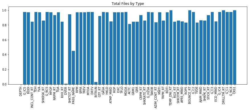
We can see that many of the channels have a large number of NaN values. This isn't necessarily a terrible thing, however it's not ideal. There are multiple ways to handle the NaN values - we can leave them as is - however many ML algorithms will struggle with NaN data. We could interpolate between values, however we need to be careful here both in terms of the acceptable length of interpolation, and knowledge that interpolation may not be accurate in the sense that data anomolies / etc may be contained in the missing values. Other options involve forward or backward fill rather than interporlation.
Pandas has a built in interpolation function call which has a limit argument. The limit is defined as number of consecutive missing datapoints to fill. From the header we can see that generally we have a 0.5ft data interval - however there are also examples where the data has a larger than 0.5ft gap. For this example we will interpolate up to 5 missing datapoints.
for col in df:
    df[col] = pd.to_numeric(df[col], errors='coerce')
df = df.interpolate(axis = 1, limit = 5)
df.head()
| DEPTH | G_IC5 | BDDI | INCL_CONT_RT | TDH | TVA | SHKRSK_RT | G_NC5 | MFOP | NRPM_RT | ... | AJAM_MWD | SHKPK_RT | STICK_RT | G_C3 | ECD_MWD | G_IC4 | DRILLTM_RT | G_C1 | G_NC4 | CRS1 | |
|---|---|---|---|---|---|---|---|---|---|---|---|---|---|---|---|---|---|---|---|---|---|
| 0 | 0.000000 | 0.000000 | 0.000000 | 0.000000 | 0.000000 | 0.000000 | NaN | NaN | NaN | NaN | ... | 601.201 | 601.201 | 601.201 | NaN | NaN | NaN | 601.201 | 601.201 | 601.201 | 601.201 |
| 1 | 300.688986 | 300.688988 | 300.688990 | 300.688992 | 300.688994 | 300.688996 | NaN | NaN | NaN | NaN | ... | NaN | NaN | NaN | NaN | NaN | NaN | NaN | NaN | NaN | NaN |
| 2 | 301.299222 | 301.299621 | 301.300020 | 301.300419 | 301.300818 | 301.301217 | NaN | NaN | NaN | NaN | ... | NaN | NaN | NaN | NaN | NaN | NaN | NaN | NaN | NaN | NaN |
| 3 | 301.610902 | 301.610578 | 301.610253 | 301.609929 | 301.609605 | 301.609280 | NaN | NaN | NaN | NaN | ... | NaN | NaN | NaN | NaN | NaN | NaN | NaN | NaN | NaN | NaN |
| 4 | 302.240823 | 302.240672 | 302.240521 | 302.240370 | 302.240219 | 302.240068 | NaN | NaN | NaN | NaN | ... | NaN | NaN | NaN | NaN | NaN | NaN | NaN | NaN | NaN | NaN |
5 rows × 58 columns
plt.figure(figsize = (15,5))
plt.bar(range(len(df.isna().sum())), list(df.isna().sum().values / len(df)), align='center')
plt.xticks(range(len(df.isna().sum())), df.columns.to_list(), rotation='vertical')
plt.title('Total Files by Type')
plt.show()
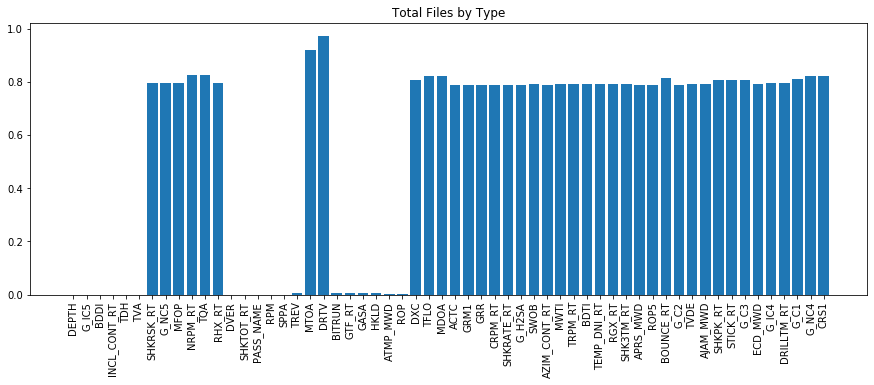
From the interpolation we can see that we dramatically reduced the missing data for many of the channels in the dataset. For those channels that still have missing data the average is closer to 80% rather than 95+%. Using this data we can now explore the data. Next week we will dive more in depth with some basic EDA - however the plot below shows what is capable given the drilling mechanics data.
import seaborn as sns
plt.figure(figsize = (10,10))
sns.scatterplot('SWOB', 'ROP', data = df)
<matplotlib.axes._subplots.AxesSubplot at 0x23e53c61240>
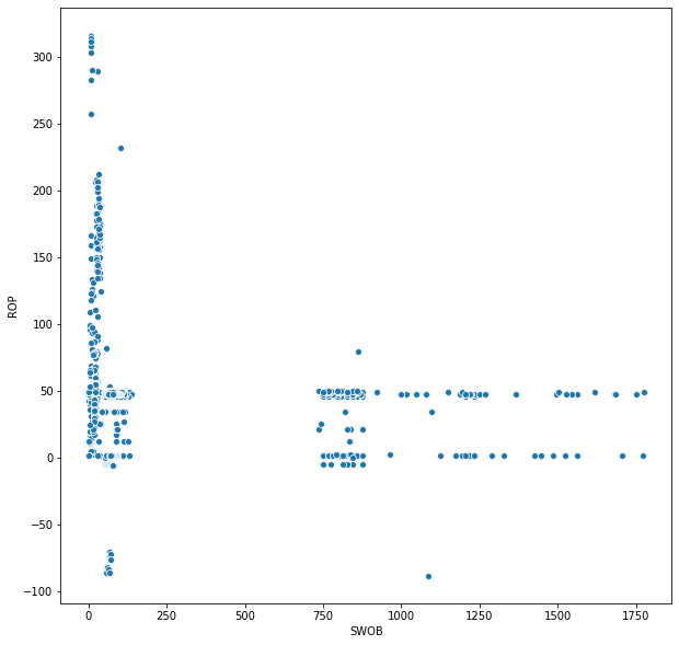
Clearly there are data quality issues with the data that we've imported. Negative ROP and/or WOB > 500 likely aren't actually correct values. This will be handled in another blog post. What I will conclude with is an example code to import and merge three different log files that contain different runs. This first file contained 10k rows of data, however that does not encompass the entire well. We need to read in multiple files and merge them to define the entire wellbore.
filename = 'WITSML Realtime drilling data/Norway-StatoilHydro-15_$47$_9-F-14/1/log/1/1/1'
blob = sas_blob_service.list_blobs('pub', filename)
master_df = pd.DataFrame()
for x, file in enumerate(blob):
    blob = sas_blob_service.get_blob_to_text('pub', file.name)
    soup = BeautifulSoup(blob.content, 'xml')
    log_names = soup.find_all('mnemonicList')
    unit_names = soup.find_all('unitList')
    header = [i + ' - ' + j for i, j in zip(log_names[0].string.split(","), unit_names[0].string.split(","))]
    data = soup.find_all('data')
    df = pd.DataFrame(columns=header,
                      data=[row.string.split(',') for row in data])
    df = df.replace('', np.NaN)
    df = units(df)
    if x == 0:
        master_df = df
    else:
        master_df = pd.concat([master_df, df], sort = False)
print('Total Length of DataFrame: ' + str(len(master_df)))
master_df.head()
Total Length of DataFrame: 30000
| DEPTH | G_IC5 | BDDI | INCL_CONT_RT | TDH | TVA | SHKRSK_RT | G_NC5 | MFOP | NRPM_RT | ... | AJAM_MWD | SHKPK_RT | STICK_RT | G_C3 | ECD_MWD | G_IC4 | DRILLTM_RT | G_C1 | G_NC4 | CRS1 | |
|---|---|---|---|---|---|---|---|---|---|---|---|---|---|---|---|---|---|---|---|---|---|
| 0 | 0.000000 | NaN | NaN | NaN | NaN | NaN | NaN | NaN | NaN | NaN | ... | NaN | NaN | NaN | NaN | NaN | NaN | 601.201 | NaN | NaN | NaN |
| 1 | 300.688986 | NaN | NaN | NaN | NaN | NaN | NaN | NaN | NaN | NaN | ... | NaN | NaN | NaN | NaN | NaN | NaN | NaN | NaN | NaN | NaN |
| 2 | 301.299222 | NaN | NaN | NaN | NaN | NaN | NaN | NaN | NaN | NaN | ... | NaN | NaN | NaN | NaN | NaN | NaN | NaN | NaN | NaN | NaN |
| 3 | 301.610902 | NaN | NaN | NaN | NaN | NaN | NaN | NaN | NaN | NaN | ... | NaN | NaN | NaN | NaN | NaN | NaN | NaN | NaN | NaN | NaN |
| 4 | 302.240823 | NaN | NaN | NaN | NaN | NaN | NaN | NaN | NaN | NaN | ... | NaN | NaN | NaN | NaN | NaN | NaN | NaN | NaN | NaN | NaN |
5 rows × 58 columns
In the code above we loaded each WITSML file individually and then combined them to create a log file of the entire wellbore. We have now successfully loaded the WITSML log based files into a pandas dataframe. There are other WITSMl files (trajectory, etc) that we will also need to import in order to effectively capture all the data in the Volve dataset - but this provides a good start, as the log based data contain a bulk of the data explaining the drilling process.
In future weeks we will explore not only depth based but time based data. We will look deeper into the logs via exploratory data analysis and discuss how to handle missing or incorrect data, and we will analyze ways in which to effectively store this data as it gets bigger. For now we only have worked with 30k rows - however if we were to involve the entire field, this would quickly reach the limit of our computers memory and could not be contained in a single pandas dataframe.