Volve Dataset Exploration

Equinor has recently released a significant amount of data pertaining to the Volve field and has made it publicly accessible. The intent of the data release is to enable others to utilize data captured over the life of field development and production. Because of the intellectual property and privacy of most of oil and gas data - it is relatively uncommon to publicly release such a large and complete volume of oil and gas data.

A little background on the Volve field. The field is located in the North Sea off the coast between Norway and the UK. It is owned and operated by Equinor (formerly Statoil) who has commissioned the release of the data. The Volve field was discovered in 1993 and approved to develop in 2005. The field saw active production between 2008 and 2016 from a total of 3 exploration wells and 21 developmental wells. Total production from the oil field was 63 million barrels of oil with a peak production rate of 56,000 bbd (barrels per day).

In total the dataset is over 5TB and includes raw data (well logs, trajectory files, seismic, drilling mechanics, etc) as well as interpreted data (geophysical interpretation from seismic, Eclipse reservoir models). Equinor is using the Azure platform to host the data and has made the dataset available within a container for easy access. Oil and gas data is frequently contained in unique types of files - whether that is WITSML (an XML document with its own standards), LAS, DLIS, excel, PDF, CSV, etc - along with software specific files such as those showing Eclipse models - a software provided by Schlumberger and commonly used for seismic data. The difficulty in finding the maximum benefit of this data is mutlifaceted: - Data using different and/or proprietary file formats makes it difficult to integrate into a 'data science' or easily ingestible and useable format - Amount of data. 5TB can rarely fit onto one hard drive let alone in memory. Large data routines (distributed computing) are becoming more and more prevalant and can help ingest and explore the data

The objective of this blog will be to walk through different aspects of exploring the Volve dataset. First gaining access to the data and exploring the data contents. Next we will explore ingesting some of the unique file formats that are frequently used in the oil and gas industry (and used in the Volve dataset). From there we will explore the data, database development, etc in an effort to apply data science prinicpals and practices to the oil and gas industry. The hope and benefit will be to expose the utility of data science in the oil and gas industry and reduce the barrier to entry of ingesting and using the data.

In order to access the data a user can: - Go to this link and register using your name and email. Then download the files locally. This can certainly be a problem not only for the time it takes to download 5TB of data (frequently including timeout while downloading a large file causing the user to need to re-download) - but also the storage constraints in order to host that amount of data - Register using the link and then using AZ copy (an azure copy method) or Azure Storage Explorer (a local program) to manage the downloading of such a large file size - Directly access the data using azure connection tools - forgoing the need to locally host/download. This is the method we will explore in this notebook. Because it's possible to use the link to forgoe registration I will remove the actual link. Once registered the user can get the URI link as given on the site referenced to be utilized to connect via Azure Storage Explorer. In order to make use of the code given here replace the sas_token as the text in the link starting with 'sv='.

Below we will connect to the container hosting the data and explore the dataset, including folder structure, file contents, etc. Future blog posts will begin to analyze some of the data and show how oil and gas data can be incorporated into a data science workflow to gain valuable insights - the intent of the data release!

# Import required libraries & packages
# from azure.kusto.data.request import KustoClient, KustoConnectionStringBuilder
# from azure.kusto.data.exceptions import KustoServiceError
# from azure.kusto.data.helpers import dataframe_from_result_table
from azure.storage.blob import BlockBlobService
import pandas as pd
import xml.etree.ElementTree as ET
from bs4 import BeautifulSoup
from collections import defaultdict
import seaborn as sns
import numpy as np
import matplotlib.pyplot as plt
%matplotlib inline

Using Blob Service to Connect to SAS

The Volve dataset as previously mentioned is hosted on Azure. Equinor has made the data read accessible via a URI link. Using the URI link we can connect to the container and begin to explore the files contained within. Below we will connect to the container and explore the dataset.

# List the account name and sas_token *** I have removed the SAS token in order to allow the user to register properly thorugh Equinor's data portal
azure_storage_account_name = 'dataplatformblvolve'
sas_token = '###'

# Create a service and use the SAS 
sas_blob_service = BlockBlobService( 
    account_name=azure_storage_account_name, 
    sas_token=sas_token,
)

filename = 'WITSML Realtime drilling data/'

blob = sas_blob_service.list_blobs('pub', filename)
blob

<azure.storage.common.models.ListGenerator at 0x7f47441001d0>

Above we used the URI link including the account name, container ('pub') and the sas token to access the account via SAS or shared access signature. This is a method a data owner can grant to users for a specified time period and allows read access only to the user. Other methods in order to access Azure Storage would use account keys and/or login information. Provided the SAS token we can connect to the Volve container and begin exploring. There are of course a number of methods and protocols to explore the dataset. On azure the list of methods that can be used to interact with blobs and containers can be found here.

In the code above we have assigned the variable 'blob' a list generator which contains all of the files contained under the 'WITSML Realtime drilling data' folder. Depicted below is a picture of the folder structure as accessed via Azure Storage Explorer. We can see there are a number of folders each of which detail a specific type of drilling data (seismic, production, logs, reports, drilling mechanics):

As printed in the first code cell - we can see that blob is a list generator - which has a different syntax than a python list. In order to access the elements of the data we have to loop through the generator. Below we will get the length of the list generator (number of files contained under all subdirectories in the WITSML Realtime drilling data folder) along with the sub-folders.

# Initialize count variable
x = 0
print_var = False
# Initialize dictionary - defaultdict initialized every key to 0
sub_dirs = defaultdict(int)
# Iterate through list generator
for b in blob:
    x+=1
    # Perform this test to avoid files directly under the WITSML folder
    if len(b.name.split('/')) > 2:
        sub_dirs[b.name.split('/')[1]] += 1
        # Not the prettiest way to show an exmample folder structure
        if not print_var and len(b.name.split('/')) > 5:
            print(b.name)
            print_var = True

print('Total Number of Files in WITSML folder: ' + str(x))
print('Total Number of Folders under WITSML folder: ' + str(len(sub_dirs)))
well_names = set(x[x.find('1'):] for x in sub_dirs.keys())
print('Total number of wells: ' + str(len(well_names)))
print('Folders contained under WITSML Folder: ')
for key in sub_dirs.keys():
    print(key)

WITSML Realtime drilling data/NA-NA-15_$47$_9-F-5/1/log/1/1/1/00001.xml
Total Number of Files in WITSML folder: 20087
Total Number of Folders under WITSML folder: 26
Total number of wells: 17
Folders contained under WITSML Folder: 
NA-NA-15_$47$_9-F-5
Norway-NA-15_$47$_9-F-1 C
Norway-NA-15_$47$_9-F-1
Norway-NA-15_$47$_9-F-11 B
Norway-NA-15_$47$_9-F-9 A
Norway-Statoil-15_$47$_9-F-12
Norway-Statoil-15_$47$_9-F-7
Norway-Statoil-NO 15_$47$_9-F-1 B
Norway-Statoil-NO 15_$47$_9-F-1 C
Norway-Statoil-NO 15_$47$_9-F-11
Norway-Statoil-NO 15_$47$_9-F-12
Norway-Statoil-NO 15_$47$_9-F-14
Norway-Statoil-NO 15_$47$_9-F-15
Norway-Statoil-NO 15_$47$_9-F-4
Norway-Statoil-NO 15_$47$_9-F-5
Norway-Statoil-NO 15_$47$_9-F-7
Norway-Statoil-NO 15_$47$_9-F-9
Norway-StatoilHydro-15_$47$_9-F-10
Norway-StatoilHydro-15_$47$_9-F-14
Norway-StatoilHydro-15_$47$_9-F-15
Norway-StatoilHydro-15_$47$_9-F-15A
Norway-StatoilHydro-15_$47$_9-F-15B
Norway-StatoilHydro-15_$47$_9-F-15S
Norway-StatoilHydro-15_$47$_9-F-4
Norway-StatoilHydro-15_$47$_9-F-5
Norway-StatoilHydro-15_$47$_9-F-9

We can see that there are over 20k files contianed in just the WITSML drilling data folder! Over the course of this blog we will ingest this data and utilize different methods to store and access all of this data.

There are a total of 26 folders under the WITSML data folder associated with a total of 17 wells. As mentioned previously the field consisted of a total of 24 drilled wells - meaning that some of the wells that were driled don't have associated WITSML data. Comparing the well names within the Volve field with the well names derived from folder structure - it appears as though the exploration wells are not represented. There are also some missing development wells such as 9-F-15D (although there is a 9-F-15S which isn't listed as a development well). This is a good moment to mention how in all field of data science but I believe particularly when looking at oil and gas datasets - the data may be missing / mislabeled / incorrect / etc. Having the proper QC guidelines in place is essential. Most of the time associated with getting a data science project off the ground will be in organizing, quality checking and synthesizing the available data in order to start painting a picture of the problem and assets.

From the example file name we can see that there are many sub-directories underneath a particular well. We will need to further explor to understand what all of these folders mean - however they likely detail runs and/or passes made during the drilling execution of the well. While drilling multiple runs are required due to multiple strings of casing / bit trips / etc. Under most sub directories we have a log folder which contains the drilling mechanics files in WITSML format, and we also have a trajectory folder which contains survey information (wellbore position) also in WITSML format. It is clear therefore that in future data exploration we will need to efficiently read WITSML data into our data science platform. This will be covered on next weeks blog.

Brief EDA of Folder Structure and File Count

plt.figure(figsize = (10,5))
plt.bar(range(len(sub_dirs)), list(sub_dirs.values()), align='center')
plt.xticks(range(len(sub_dirs)), list(sub_dirs.keys()), rotation='vertical')
plt.show()

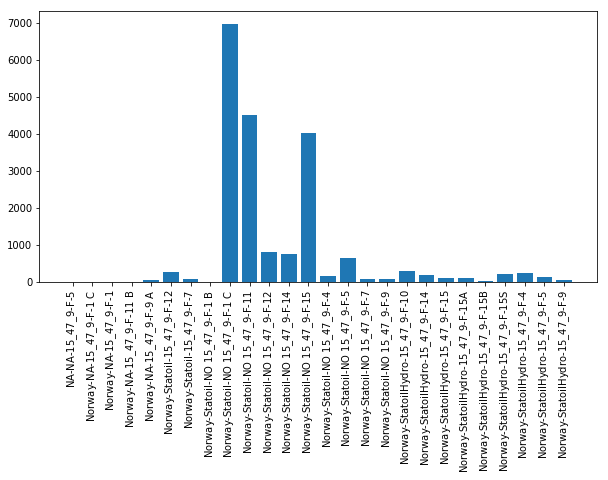
Above we have plotted the number of files under each of the 26 sub-folders previously mentioned. We can see that we have a fairly uneven dataset where 3 wells comprise > 75% of the entire file count. What this may mean is that other wells won't necessarily contain complete information related to the construction of the wellbore - or it may mean that most wells were completed in relatively few runs and therefore the total file count is lower but there is more information contained in each file (will explore below). Exploring some of the sub-folders we can see that many comprise only log and trajectory data (as previously detailed) but others are more complete (including those wells listed with higher file count:

This folder structure (where available) will help to better characterize the construction process undertaken for that well. Below we analyze the average file size for each sub-folder.

# A list generator can only be iterated over once - so we have to re-query the Azure Storage
blob = sas_blob_service.list_blobs('pub', filename)
# Initialize dictionary - defaultdict initialized every key to 0
sub_dirs_length = defaultdict(int)
# Iterate through list generator
for b in blob:
    x+=1
    # Perform this test to avoid files directly under the WITSML folder
    if len(b.name.split('/')) > 2:
        # Total the blob size in bytes
        sub_dirs_length[b.name.split('/')[1]] += b.properties.content_length

plt.figure(figsize = (10,5))
plt.bar(range(len(sub_dirs_length)), list(sub_dirs_length.values()), align='center')
plt.xticks(range(len(sub_dirs_length)), list(sub_dirs_length.keys()), rotation='vertical')
plt.title('Total Folder Size by Folder')
plt.show()

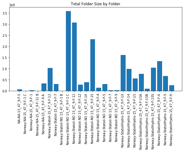
The plot above looks at the total content size underneath each folder. This appears to closely match the total file count depicted above - however we can see that some of the wells (particularly those on the right hand size of the x-axis) have a larger folder size. This is promising that there may be more information contained on a number of wells due to a larger file size. Below we analyze average file size by folder.

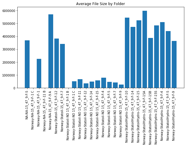
# Loop through keys and divide by number of files (from previous code cell)
for key in sub_dirs_length.keys():
    sub_dirs_length[key] = sub_dirs_length[key] / sub_dirs[key]

plt.figure(figsize = (10,5))
plt.bar(range(len(sub_dirs_length)), list(sub_dirs_length.values()), align='center')
plt.xticks(range(len(sub_dirs_length)), list(sub_dirs_length.keys()), rotation='vertical')
plt.title('Average File Size by Folder')
plt.show()

So far we have only looked at a subset of the Volve dataset contained in the 'WITSML' folder. This has been in order to narrow the focus of our investigation (not to mention the time to query the entire dataset). However it is also important to understand that each of the primary folders contains different types of data that helps explain the Volve field. Integration of all of this information will be critical in order to most beneficially understand the field. Below we look at a count by file type over the entire Volve field.

# Look at all files in Volve Dataset
blob = sas_blob_service.list_blobs('pub')
# Initialize dictionary - defaultdict initialized every key to 0
file_type = defaultdict(int)
# Iterate through list generator
for b in blob:
    # Perform this test to avoid folder structures
    if len(b.name.split('.')[-1]) < 10:
        # Total count of file type
        file_type[b.name.split('.')[-1]] += 1
# Filter for only file types having count > 1
file_type_filter = {}
for (key, value) in file_type.items():
    if value > 1:
        file_type_filter[key] = value

plt.figure(figsize = (10,5))
plt.bar(range(len(file_type_filter)), list(file_type_filter.values()), align='center')
plt.xticks(range(len(file_type_filter)), list(file_type_filter.keys()), rotation='vertical')
plt.title('Total Files by Type')
plt.show()

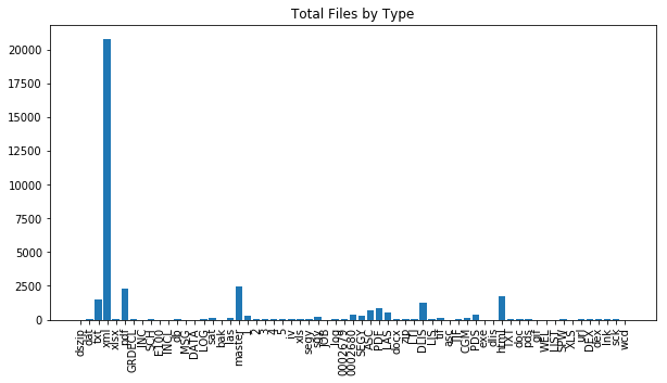
From the plot above we can see that XML overwhelmingly has the largest count of files. This is likely the WITSML file type that was previously discussed and will more thoroughly be examined next week. Beyond WITSML there are some other files associated with text, html, LAS. The variance in terms of file type is one of the challenges in all data science projects - but particularly true in the oil and gas industry.

Wrapping it Up & Next Week

We have taken a very introductory look into the Volve dataset - the folder structure and file types involved. There are certainly a number of challenges involved in ingesting the data that has been released: - Volume of the data - File types and data extraction. This will require domain specific knowledge, writing functions to import some of the oil and gas data types and an efficient storage structure to contain all the data - Missing data. As shown above some wells have a large volume of data while others appears to be absent from the dataset and/or contain little information. These wells will be more difficult to fully characterize

We have explored using the blob connection to directly query azure storage which is much more efficient that downloading all files contained in the dataset. There are a number of other methods that can be used to further explore azure blob connections and the Volve dataset and I encourage you to look over this site to better understand how to get information from the azure storage blob and container. You can always also type ? object in a jupyter code cell and execute in order to get the documentation associated with that object which may reveal available methods to be used.

Next week will will start looking at ingesting the data - specifically WISTML files. This is a custom file type specific to the oil and gas industry. Energistics (the company that maintains the standards of WITSML) has developed an API in .NET and there are other available resources to use JAVA to work with this data. Because both of these programming languages aren't traditionally used in data science we will write our own xml parser to look as some of the files and work with the ingested data. Future work will involve converting these libraries into a python friendly format so that all of the classes/methods and newly developed standards can be incorporated.

Until then happy exploring the Volve dataset and getting your hands dirty incorporating data science practices in your oil and gas dataset!