Reading In Other WITSML
To date we have shown how to read in WITSML log files - or files with an xml ending that follow the WITSML standard and contain log (date or time) based data. We have written import functions to read in the WTSML log data. In another week we will utilize a java based SDK which follows Energistics standards for reading in xml data (rather than our custom written parser). However in the mean time - while log data is extremely impactful for understanding the fundamentals of drilling and/or rock properties/mechanics, there are a number of other WITSML data types that compose essential data that may (or may not) be impactful on the drilling and rock property measurements.
Two common other types of WITSML data are trajectory files and BHA's. Trajectory contains the surveys (typically at approximately 100' intervals) giving at a minimum the measured depth, inclination and azimuth. Many other trajectory files also give additional information such as true vertical depth (TVD), dogleg severity (DLS), build and/or turn rate, as well as other measurements based on the surface location (Northing/Easting, Latitude/Longitude, etc). Knowing the trajectory is essential both for understanding the drilling process (low ROP but high DLS may indicate sliding in a curve section), as well as the rock properties measured (resistivity horn observed while drilling at a high angle can signify crossing a bed boundary). BHA information gives a record of the bottom hole assembly used to drill a particular section. BHA data can give an indication as to the method to control wellbore deviation (rotary assembly, motor, rotary steerable, etc) as well as the distance to bit for many measurement types (LWD/MWD), and finally the stabilizer/reamer placement which may control wellbore deviation, hole size and a number of other properties.
This week we will set out to read in these two types of information and utlize the data contained in both to merge into our log files to give a more complete picture of the drilling environment.
# Import required libraries & packages
from azure.storage.blob import BlockBlobService
import pandas as pd
import xml.etree.ElementTree as ET
from bs4 import BeautifulSoup
from collections import defaultdict
import seaborn as sns
import numpy as np
import matplotlib.pyplot as plt
%matplotlib inline
import os
import glob
# List the account name and sas_token *** I have removed the SAS token in order to allow the user to register properly thorugh Equinor's data portal
azure_storage_account_name = 'dataplatformblvolve'
sas_token = 'sv=2018-03-28&sr=c&sig=yqAsIUqdM4HZx8K7QAksMeyueJ00esylOSHh4RgkQc4%3D&se=2020-05-26T21%3A55%3A41Z&sp=rl'

# Create a service and use the SAS
sas_blob_service = BlockBlobService(
    account_name=azure_storage_account_name,
    sas_token=sas_token,
)

filename = 'WITSML Realtime drilling data/Norway-Statoil-NO 15_$47$_9-F-4/1'

blob = sas_blob_service.list_blobs('pub', filename)
for x, b in enumerate(blob):
    print(b.name)
    if x > 10:
        break
WITSML Realtime drilling data/Norway-Statoil-NO 15_$47$_9-F-4/1/_wellboreInfo/NO 15_$47$_9-F-4 (dbffce7a-74d8-4443-8b7e-b937e5fede95)(NULL).xml
WITSML Realtime drilling data/Norway-Statoil-NO 15_$47$_9-F-4/1/bhaRun/1.xml
WITSML Realtime drilling data/Norway-Statoil-NO 15_$47$_9-F-4/1/bhaRun/2.xml
WITSML Realtime drilling data/Norway-Statoil-NO 15_$47$_9-F-4/1/bhaRun/3.xml
WITSML Realtime drilling data/Norway-Statoil-NO 15_$47$_9-F-4/1/bhaRun/4.xml
WITSML Realtime drilling data/Norway-Statoil-NO 15_$47$_9-F-4/1/bhaRun/MetaDataFileInfo.txt
WITSML Realtime drilling data/Norway-Statoil-NO 15_$47$_9-F-4/1/log/1/1/1/00001.xml
WITSML Realtime drilling data/Norway-Statoil-NO 15_$47$_9-F-4/1/log/1/1/1/00002.xml
WITSML Realtime drilling data/Norway-Statoil-NO 15_$47$_9-F-4/1/log/1/1/1/00003.xml
WITSML Realtime drilling data/Norway-Statoil-NO 15_$47$_9-F-4/1/log/1/1/1/00004.xml
WITSML Realtime drilling data/Norway-Statoil-NO 15_$47$_9-F-4/1/log/1/1/1/00005.xml
WITSML Realtime drilling data/Norway-Statoil-NO 15_$47$_9-F-4/1/log/1/1/1/00006.xml
def units(df):
    '''
    The intent of this function is to convert units from metric to US

    Input: df - pandas dataframe
    Output: df - pandas dataframe with columns transformed based on current units

    '''
    corr_columns = []
    for col in df.columns:
        corr_columns.append(col.split(' - ')[0])
        try:
            df[col] = df[col].astype(float)
        except:
            continue
        # Analyze column units and transform if appropriate
        # Future work will use dictionary rather than series of if statements
        if (col.split(' - ')[1] == 'm') | (col.split(' - ')[1] == 'm/h') | (col.split(' - ')[1] == 'm/s2'):
            df[col] = df[col].astype(float) * 3.28084
        if col.split(' - ')[1] == 'degC':
            df[col] = (df[col].astype(float) * 9/5) + 32
        if col.split(' - ')[1] == 'm3':
            df[col] = df[col].astype(float) * 6.289814
        if col.split(' - ')[1] == 'kkgf':
            df[col] = df[col].astype(float) * 2.2
        if col.split(' - ')[1] == 'kPa':
            df[col] = df[col].astype(float) * 0.145038
        if col.split(' - ')[1] == 'L/min':
            df[col] = df[col].astype(float) * 0.264172875
        if col.split(' - ')[1] == 'g/cm3':
            df[col] = df[col].astype(float) * 8.3454
        if col.split(' - ')[1] == 'kN.m':
            df[col] = df[col].astype(float) * 0.737562

    df.columns = corr_columns
    return df
BHA
The code above was replicated from prior weeks. Below we will take an example BHA WITSML file and parse appropriately. In the folder we are working out of, the BHA's only contain a single tubular compponent listed under the 'tubular' tag - see below for a list of the tags.
filename = 'WITSML Realtime drilling data/Norway-Statoil-NO 15_$47$_9-F-4/1/bhaRun/3.xml'
blob = sas_blob_service.get_blob_to_text('pub', filename)
soup = BeautifulSoup(blob.content, 'xml')
for tag in soup.find_all():
    print(tag.name)
    if tag.name == 'tubular':
        print(tag.text)
bhaRuns
bhaRun
nameWell
nameWellbore
name
tubular
15/9-F-4_16VIRG33
dTimStart
numStringRun
commonData
sourceName
dTimCreation
dTimLastChange
itemState
comments
priv_userLastChange
priv_ipLastChange
priv_userOwner
priv_ipOwner
priv_dTimReceived
Above we printed all of the tags contained in teh BHA WITSML file - most of which contain the logging information for the creation of the file. There is however a couple of notable tags that will be required to combine the BHA information with the logging data: bhaRun, nameWell, and tubular.
- bhaRun - contains the uid (unique indentification) for the BHA run - which will give the user the start/stop time and depth for the run. Using this information the BHA contents can be appended to the logging data approrpriately.
- nameWell - name of the well - given the folder/file structure of the Volve dataset, this is also contained in the folder naming - however when combining multiple wells it is essential to keep track of this data
- tubular - a reference to the tubular catalog for the well listed under the 'tubular' directory. We will use this infomration in order to look up the correct tubular.
As was printed above, the name of the tubular for this particular bha run is 16VIRG33 - we will use this to get the data associated with this tubular. If the BHA contained more detailed information - additional tubulars would be present here as well. Lets load the tubular file and inspect the qualities of that component.
filename = 'WITSML Realtime drilling data/Norway-Statoil-NO 15_$47$_9-F-4/1/tubular/1.xml'
blob = sas_blob_service.get_blob_to_text('pub', filename)
soup = BeautifulSoup(blob.content, 'xml')
for tag in soup.find_all():
    print(tag.name + ': ' + tag.text)
tubulars: NO 15/9-F-4NO 15/9-F-415/9-F-4_16VIRG33drillingdrill pipe20.1213612000001770.13970000000020456240.130unknownBHIDPDrill pipetubing10.157480000000230.17780000000026205411.810unknownBHITbgTubingBaker Hughes2016-10-05T00:24:47.761Z2016-10-05T00:24:47.761Zactualsc-sync-bhi143.97.229.42016-10-05T00:24:47.761Z
tubular: NO 15/9-F-4NO 15/9-F-415/9-F-4_16VIRG33drillingdrill pipe20.1213612000001770.13970000000020456240.130unknownBHIDPDrill pipetubing10.157480000000230.17780000000026205411.810unknownBHITbgTubingBaker Hughes2016-10-05T00:24:47.761Z2016-10-05T00:24:47.761Zactualsc-sync-bhi143.97.229.42016-10-05T00:24:47.761Z
nameWell: NO 15/9-F-4
nameWellbore: NO 15/9-F-4
name: 15/9-F-4_16VIRG33
typeTubularAssy: drilling
tubularComponent: drill pipe20.1213612000001770.13970000000020456240.130unknownBHIDPDrill pipe
typeTubularComp: drill pipe
sequence: 2
id: 0.121361200000177
od: 0.139700000000204
len: 562
lenJointAv: 40.1
numJointStand: 3
tensYield: 0
configCon: unknown
vendor: BHI
customData: DPDrill pipe
mwdComponent: DPDrill pipe
shortName: DP
fullName: Drill pipe
tubularComponent: tubing10.157480000000230.17780000000026205411.810unknownBHITbgTubing
typeTubularComp: tubing
sequence: 1
id: 0.15748000000023
od: 0.17780000000026
len: 2054
lenJointAv: 11.8
numJointStand: 1
tensYield: 0
configCon: unknown
vendor: BHI
customData: TbgTubing
mwdComponent: TbgTubing
shortName: Tbg
fullName: Tubing
commonData: Baker Hughes2016-10-05T00:24:47.761Z2016-10-05T00:24:47.761Zactualsc-sync-bhi143.97.229.42016-10-05T00:24:47.761Z
sourceName: Baker Hughes
dTimCreation: 2016-10-05T00:24:47.761Z
dTimLastChange: 2016-10-05T00:24:47.761Z
itemState: actual
priv_userOwner: sc-sync-bhi
priv_ipOwner: 143.97.229.4
priv_dTimReceived: 2016-10-05T00:24:47.761Z
Inspecting the tubular data, there appears to be two kinds of tubulars under the 16VIRG33 tubular identification: - Drill Pipe - Tubing
It's possible this was a tubing while drilling run, or it may be two BHA's one for drilling another for casing - however under the tubular node, for typeTubularAssy we can see 'drilling' meaning most likely this BHA was intended for drilling. For each tubular componnent we can see some key peices of information - for instance under drill pipe we can see: - OD/ID information (OD listed as 0.1397m or 5.5") - Total length as well as average join length and number of joints per stand
In order to meaningfully link the tubular components back to the logs we need the wellbore geometry data to link the tubular/BHA name to the sections drilled. Below we inspect the WBG file for this run:
filename = 'WITSML Realtime drilling data/Norway-Statoil-NO 15_$47$_9-F-4/1/wbGeometry/1.xml'
blob = sas_blob_service.get_blob_to_text('pub', filename)
soup = BeautifulSoup(blob.content, 'xml')
for tag in soup.find_all():
    print(tag.name + ': ' + tag.text)
wbGeometrys: NO 15/9-F-4NO 15/9-F-415/9-F-42016-09-30T10:05:00.000Z3510091casing593263059326300.2167890000003170.244475000000357riser0200200.5080000000007420.558800000000816open hole26303510263035100.17780000000026casing20593205930.2453640000003580.273050000000399Baker Hughes2016-09-30T11:36:13.275Z2016-09-30T18:51:17.766Zactualsc-sync-bhi143.97.229.4statfeedstg10.166.14.62016-09-30T18:47:26.377Z
wbGeometry: NO 15/9-F-4NO 15/9-F-415/9-F-42016-09-30T10:05:00.000Z3510091casing593263059326300.2167890000003170.244475000000357riser0200200.5080000000007420.558800000000816open hole26303510263035100.17780000000026casing20593205930.2453640000003580.273050000000399Baker Hughes2016-09-30T11:36:13.275Z2016-09-30T18:51:17.766Zactualsc-sync-bhi143.97.229.4statfeedstg10.166.14.62016-09-30T18:47:26.377Z
nameWell: NO 15/9-F-4
nameWellbore: NO 15/9-F-4
name: 15/9-F-4
dTimReport: 2016-09-30T10:05:00.000Z
mdBottom: 3510
gapAir: 0
depthWaterMean: 91
wbGeometrySection: casing593263059326300.2167890000003170.244475000000357
typeHoleCasing: casing
mdTop: 593
mdBottom: 2630
tvdTop: 593
tvdBottom: 2630
idSection: 0.216789000000317
odSection: 0.244475000000357
wbGeometrySection: riser0200200.5080000000007420.558800000000816
typeHoleCasing: riser
mdTop: 0
mdBottom: 20
tvdTop: 0
tvdBottom: 20
idSection: 0.508000000000742
odSection: 0.558800000000816
wbGeometrySection: open hole26303510263035100.17780000000026
typeHoleCasing: open hole
mdTop: 2630
mdBottom: 3510
tvdTop: 2630
tvdBottom: 3510
idSection: 0.17780000000026
wbGeometrySection: casing20593205930.2453640000003580.273050000000399
typeHoleCasing: casing
mdTop: 20
mdBottom: 593
tvdTop: 20
tvdBottom: 593
idSection: 0.245364000000358
odSection: 0.273050000000399
commonData: Baker Hughes2016-09-30T11:36:13.275Z2016-09-30T18:51:17.766Zactualsc-sync-bhi143.97.229.4statfeedstg10.166.14.62016-09-30T18:47:26.377Z
sourceName: Baker Hughes
dTimCreation: 2016-09-30T11:36:13.275Z
dTimLastChange: 2016-09-30T18:51:17.766Z
itemState: actual
priv_userLastChange: sc-sync-bhi
priv_ipLastChange: 143.97.229.4
priv_userOwner: statfeedstg
priv_ipOwner: 10.166.14.6
priv_dTimReceived: 2016-09-30T18:47:26.377Z
Putting our BHA/Tubular/WBG inspection workflow together, we can see that the wbGeometrySection has a uid linked to the bhaRun which is also linked to the tubular uid. In this example we only had drill pipe in the BHA - therefore the benefit gained from BHA will be limited - because the BHA is incomplete (most likely since all BHA's need a bit). We can use the top and bottom TVD and md information to better understand where this run took place in the well construction phase and then incoroporate key BHA information into our logging dataframe (things such as bit size (could also directly be read from the WBG file), number of stabilizers, BHA type (rotary, motor, RSS), as well as any number of other key pieces of information.
Trajectory Incorporation
Next we will begin to inspect the trajectory WITSML files in order to link logging data to trajectory information. First we will inspect the trajectory file:
filename = 'WITSML Realtime drilling data/Norway-Statoil-NO 15_$47$_9-F-4/1/trajectory/1.xml'
blob = sas_blob_service.get_blob_to_text('pub', filename)
soup = BeautifulSoup(blob.content, 'xml')
for tag in soup.find_all('trajectory'):
    continue
tag.findChildren()[:16]
[<nameWell>NO 15/9-F-4</nameWell>,
 <nameWellbore>NO 15/9-F-4</nameWellbore>,
 <name>MWD-15/9-F-4</name>,
 <objectGrowing>false</objectGrowing>,
 <dTimTrajStart>2016-09-30T09:59:00.000Z</dTimTrajStart>,
 <dTimTrajEnd>2016-09-30T10:16:10.000Z</dTimTrajEnd>,
 <mdMn uom="m">0</mdMn>,
 <mdMx uom="m">3510</mdMx>,
 <magDeclUsed uom="rad">0</magDeclUsed>,
 <gridCorUsed uom="rad">0</gridCorUsed>,
 <aziVertSect uom="rad">0</aziVertSect>,
 <dispNsVertSectOrig uom="m">0</dispNsVertSectOrig>,
 <dispEwVertSectOrig uom="m">0</dispEwVertSectOrig>,
 <aziRef>true north</aziRef>,
 <trajectoryStation uid="5VIRG33_TIE_POINT"><dTimStn>2016-09-30T09:59:00.000Z</dTimStn><typeTrajStation>tie in point</typeTrajStation><md uom="m">0</md><tvd uom="m">0</tvd><incl uom="rad">0</incl><azi uom="rad">0</azi><dispNs uom="m">0</dispNs><dispEw uom="m">0</dispEw><vertSect uom="m">0</vertSect><dls uom="rad/m">0</dls><commonData><sourceName>Baker Hughes</sourceName><dTimCreation>2016-09-30T11:36:15.398Z</dTimCreation><dTimLastChange>2016-09-30T11:36:15.398Z</dTimLastChange><itemState>actual</itemState></commonData></trajectoryStation>,
 <dTimStn>2016-09-30T09:59:00.000Z</dTimStn>]
From the header information in the trajectory file we get various parameters for the wellbore, such as azimuth reference, start and end time and depth values, magnetic declination and grid correction. This information is helpful in ensuring the surveys are correctly referenced. Each survey station is then contained in the trajectoryStation node (only the first is printed here for reference). In a trajectory station there are nodes such as MD, Inc, Azi, TVD, N, E, VS. From these measurements the trajectory of the wellbore can be determined. Other features such as DLS, BR, TR, etc can be computed from these survey stations. Below we will read in all survey stations and write them to a pandas dataframe.
filename = 'WITSML Realtime drilling data/Norway-Statoil-NO 15_$47$_9-F-4/1/trajectory/1.xml'
blob = sas_blob_service.get_blob_to_text('pub', filename)
soup = BeautifulSoup(blob.content, 'xml')

md = []
inc = []
azi = []
tvd = []
for tag in soup.find_all('trajectoryStation'):
    md.append(float(tag.find('md').text) * 3.28084)
    inc.append(float(tag.find('incl').text) * 57.2958)
    azi.append(float(tag.find('azi').text) * 57.2958)
    tvd.append(float(tag.find('tvd').text) * 3.28084)
df_survey = pd.DataFrame({'md': md,
                         'inc': inc,
                         'azi': azi,
                         'tvd': tvd})
df_survey.head()
| md | inc | azi | tvd | |
|---|---|---|---|---|
| 0 | 0.000000 | 0.00 | 0.000000 | 0.000000 |
| 1 | 2.952756 | 0.00 | 0.000000 | 2.952756 |
| 2 | 604.068245 | 0.10 | 233.250083 | 604.067940 |
| 3 | 736.384528 | 0.16 | 227.580083 | 736.383877 |
| 4 | 868.733652 | 0.84 | 218.680071 | 868.727195 |
For a few other meaniningful meausrements we can add build rate, turn rate and DLS. DLS computation can be quite complex and depends on the method used - most today use the minimum curvature method. The DLS via minimum curvature can be computed:
\begin{equation} DLS = cos^{-1} * [{sin(I_1) * sin(I_2) * cos(A_2-A_1)} + {cos(I_1)cos(I_2)}] \end{equation*}
We will write a helper function for this then step through the pandas dataframe to compute these. Because we need references to two rows, we cannot use the apply function - unfortunately the iterrows is slow - but given the size of the survey file should run fairly quick.
import math
def compute_dls(inc2, inc1, azi2, azi1, md2, md1):
#     print(inc2, inc1, azi2, azi1, md2, md1)
    part1 = np.sin(inc1) * np.sin(inc2) * np.cos(azi2-azi1)
    part2 = np.cos(inc1) * np.cos(inc2)

    return np.arccos(part1 + part2) * 100 / (md2-md1)

br = [0]
tr = [0]
dls = [0]

for x, row in df_survey.iterrows():
    if x == 0:
        continue #because no prior survey to compute dls
    else:
        br.append((row['inc'] - df_survey.iloc[x-1,:]['inc']) / (row['md'] - df_survey.iloc[x-1,:]['md']) * 100)
        tr.append((row['azi'] - df_survey.iloc[x-1,:]['azi']) / (row['md'] - df_survey.iloc[x-1,:]['md']) * 100)
        dls.append(compute_dls(row['inc'], df_survey.iloc[x-1,:]['inc'], row['azi'], df_survey.iloc[x-1,:]['azi'], row['md'], df_survey.iloc[x-1,:]['md']))

df_survey['dls'] = dls
df_survey['br'] = br
df_survey['tr'] = tr

df_survey.head()
| md | inc | azi | tvd | dls | br | tr | |
|---|---|---|---|---|---|---|---|
| 0 | 0.000000 | 0.00 | 0.000000 | 0.000000 | 0.000000 | 0.000000 | 0.000000 |
| 1 | 2.952756 | 0.00 | 0.000000 | 2.952756 | 0.000000 | 0.000000 | 0.000000 |
| 2 | 604.068245 | 0.10 | 233.250083 | 604.067940 | 0.016636 | 0.016636 | 38.802874 |
| 3 | 736.384528 | 0.16 | 227.580083 | 736.383877 | 0.073280 | 0.045346 | -4.285187 |
| 4 | 868.733652 | 0.84 | 218.680071 | 868.727195 | 0.741154 | 0.513793 | -6.724648 |
We now have our trajectory in a pandas dataframe and have computed DLS, BR and TR. We can now vizualize this trajectory:
plt.figure(figsize=(20,10))
sns.lineplot(x='md', y='inc', data = df_survey)
sns.lineplot(x='md', y='azi', data = df_survey)
plt.title('Norway-Statoil-NO 15_$47$_9-F-4 Trajectory')
Text(0.5, 1.0, 'Norway-Statoil-NO 15_$47$_9-F-4 Trajectory')
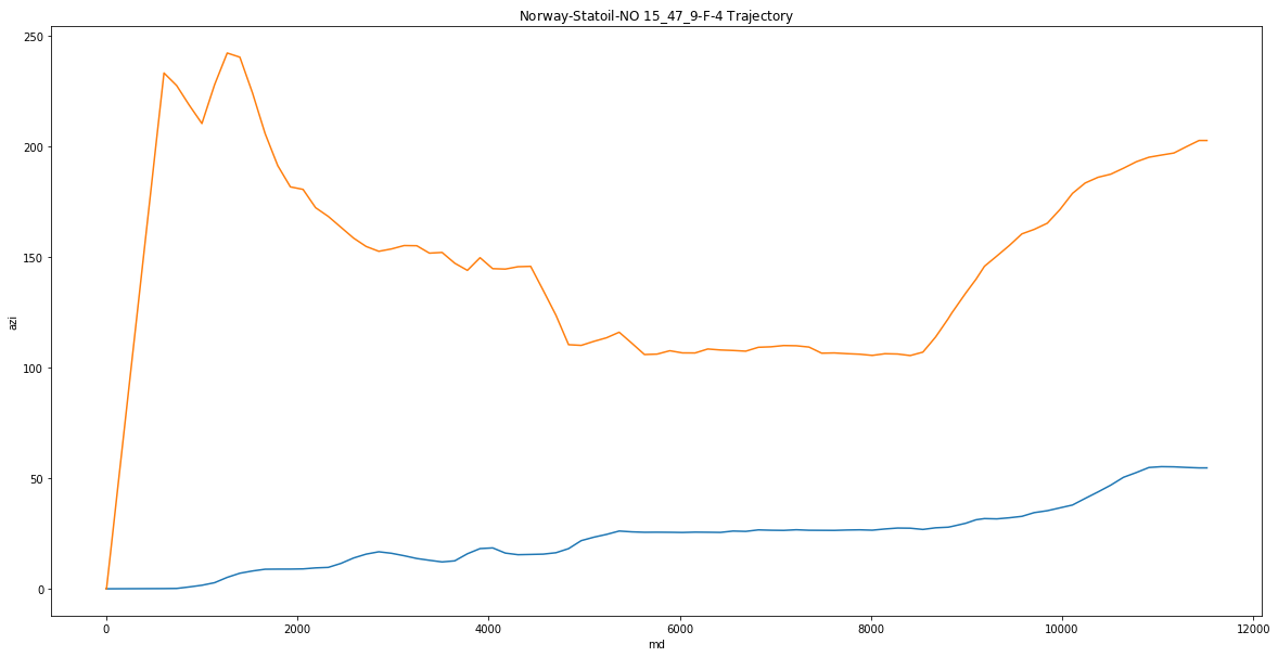
As can be seen - over the course of the well, the inclination built to a ~35deg tangent and then built again towards TD. Azimuth initially started towards the west, turnned south and held the tangent then turned back towards the west. This information will be important to include with the logging information (traejctory may have some impact on the logging data (resistivity log can be affected by how the trajectory crosses a bed boundary - computing TVD from the logging data for rock measurements, etc).
Below we read in the logging data using the code from before and then merge the two dataframes together to combine.
filename = 'WITSML Realtime drilling data/Norway-Statoil-NO 15_$47$_9-F-4/1/log/1/4/1'
blob = sas_blob_service.list_blobs('pub', filename)
master_df = pd.DataFrame()
for x, file in enumerate(blob):
    blob = sas_blob_service.get_blob_to_text('pub', file.name)
    soup = BeautifulSoup(blob.content, 'xml')
    log_names = soup.find_all('mnemonicList')
    unit_names = soup.find_all('unitList')
    header = [i + ' - ' + j for i, j in zip(log_names[0].string.split(","), unit_names[0].string.split(","))]
    data = soup.find_all('data')
    df = pd.DataFrame(columns=header,
                      data=[row.string.split(',') for row in data])
    df = df.replace('', np.NaN)
    df = units(df)
    if x == 0:
        master_df = df
    else:
        master_df = pd.concat([master_df, df], join = 'outer', sort = False)

master_df.head()
master_df['Depth'] = master_df['Depth'].round(0)
depth_df = master_df.groupby(['Depth']).mean()
depth_df.head()
| INSLIPS_STATUS | EditFlag | PIT_TRIPOUT | RigActivityCode | TRIPINSLIPS | TRIPOUTSLIPS | TRIPEXPFILL | TRIPEXPPVT | BLOCKCOMP | STANDSTOGO | ... | JOINTSDONE | FLOWOUT | PIT_TRIPIN | TRIPPULL | FLOWOUTPC | TRIPREAMFLAG | TRIPPVT | TRIPCFILL | HKLD | TRIPCEXPFILL | |
|---|---|---|---|---|---|---|---|---|---|---|---|---|---|---|---|---|---|---|---|---|---|
| Depth | |||||||||||||||||||||
| -131.0 | 0.0 | 0.0 | 39.039450 | 114.0 | 74059.0 | 101.0 | 0.048864 | 22.416786 | 57.117456 | 17.0 | ... | 10.0 | 0.000621 | 39.039450 | 0.084786 | 0.0 | 0.0 | 39.026784 | 0.0 | 823496.500000 | 0.0 |
| -100.0 | 0.0 | 0.0 | 35.531888 | 114.0 | 73922.0 | 101.0 | 0.048864 | 22.416786 | 86.205209 | 17.0 | ... | 10.0 | 0.000639 | 35.531888 | 0.084786 | 0.0 | 0.0 | 35.462372 | 0.0 | 718690.000000 | 0.0 |
| -80.0 | 0.0 | 0.0 | 32.000392 | 17.0 | 33282.0 | 88.0 | 0.032899 | 30.945326 | 89.522444 | 18.0 | ... | 9.0 | 0.000595 | 32.000392 | 0.332143 | 0.0 | 0.0 | 32.030260 | 0.0 | 815804.300000 | 0.0 |
| -77.0 | 0.0 | 0.0 | 31.309085 | 114.0 | 73710.0 | 101.0 | 0.048864 | 22.416786 | 83.469865 | 17.0 | ... | 10.0 | 0.000641 | 31.309085 | 0.084786 | 0.0 | 0.0 | 31.241690 | 0.0 | 734395.016667 | 0.0 |
| -69.0 | 0.0 | 0.0 | 32.754235 | 17.0 | 33282.0 | 58.0 | 0.032899 | 30.945326 | 78.252398 | 18.0 | ... | 9.0 | 0.000573 | 32.754235 | 0.332143 | 0.0 | 0.0 | 32.796441 | 0.0 | 804265.700000 | 0.0 |
5 rows × 25 columns
df_survey = df_survey.rename(columns={'md':'Depth'})
df_survey['Depth'] = df_survey['Depth'].round(0)
df_survey = df_survey.set_index('Depth')
df_survey.head()
| inc | azi | tvd | dls | br | tr | |
|---|---|---|---|---|---|---|
| Depth | ||||||
| 0.0 | 0.00 | 0.000000 | 0.000000 | 0.000000 | 0.000000 | 0.000000 |
| 3.0 | 0.00 | 0.000000 | 2.952756 | 0.000000 | 0.000000 | 0.000000 |
| 604.0 | 0.10 | 233.250083 | 604.067940 | 0.016636 | 0.016636 | 38.802874 |
| 736.0 | 0.16 | 227.580083 | 736.383877 | 0.073280 | 0.045346 | -4.285187 |
| 869.0 | 0.84 | 218.680071 | 868.727195 | 0.741154 | 0.513793 | -6.724648 |
df = depth_df.join(df_survey, sort = False)
df.head(10)
| INSLIPS_STATUS | EditFlag | PIT_TRIPOUT | RigActivityCode | TRIPINSLIPS | TRIPOUTSLIPS | TRIPEXPFILL | TRIPEXPPVT | BLOCKCOMP | STANDSTOGO | ... | TRIPPVT | TRIPCFILL | HKLD | TRIPCEXPFILL | inc | azi | tvd | dls | br | tr | |
|---|---|---|---|---|---|---|---|---|---|---|---|---|---|---|---|---|---|---|---|---|---|
| Depth | |||||||||||||||||||||
| -131.0 | 0.0 | 0.0 | 39.039450 | 114.0 | 74059.0 | 101.000000 | 0.048864 | 22.416786 | 57.117456 | 17.0 | ... | 39.026784 | 0.0 | 8.234965e+05 | 0.0 | NaN | NaN | NaN | NaN | NaN | NaN |
| -100.0 | 0.0 | 0.0 | 35.531888 | 114.0 | 73922.0 | 101.000000 | 0.048864 | 22.416786 | 86.205209 | 17.0 | ... | 35.462372 | 0.0 | 7.186900e+05 | 0.0 | NaN | NaN | NaN | NaN | NaN | NaN |
| -80.0 | 0.0 | 0.0 | 32.000392 | 17.0 | 33282.0 | 88.000000 | 0.032899 | 30.945326 | 89.522444 | 18.0 | ... | 32.030260 | 0.0 | 8.158043e+05 | 0.0 | NaN | NaN | NaN | NaN | NaN | NaN |
| -77.0 | 0.0 | 0.0 | 31.309085 | 114.0 | 73710.0 | 101.000000 | 0.048864 | 22.416786 | 83.469865 | 17.0 | ... | 31.241690 | 0.0 | 7.343950e+05 | 0.0 | NaN | NaN | NaN | NaN | NaN | NaN |
| -69.0 | 0.0 | 0.0 | 32.754235 | 17.0 | 33282.0 | 58.000000 | 0.032899 | 30.945326 | 78.252398 | 18.0 | ... | 32.796441 | 0.0 | 8.042657e+05 | 0.0 | NaN | NaN | NaN | NaN | NaN | NaN |
| -61.0 | 0.0 | 0.0 | 38.635193 | 106.0 | 787.0 | 3916.826087 | 0.001766 | 36.231095 | 64.410478 | 215.0 | ... | 38.635027 | 0.0 | 1.535639e+06 | 0.0 | NaN | NaN | NaN | NaN | NaN | NaN |
| -60.0 | 0.0 | 0.0 | 26.796568 | 114.0 | 73455.0 | 101.000000 | 0.048864 | 22.416786 | 109.828752 | 17.0 | ... | 26.768646 | 0.0 | 6.970022e+05 | 0.0 | NaN | NaN | NaN | NaN | NaN | NaN |
| -57.0 | 0.0 | 0.0 | 38.731530 | 106.0 | 787.0 | 4967.000000 | 0.001766 | 36.231095 | 60.745048 | 215.0 | ... | 38.731530 | 0.0 | 1.450412e+06 | 0.0 | NaN | NaN | NaN | NaN | NaN | NaN |
| -56.0 | 0.0 | 0.0 | 38.463484 | 106.0 | 787.0 | 1562.056818 | 0.001766 | 36.231095 | 59.007515 | 215.0 | ... | 38.463568 | 0.0 | 1.533059e+06 | 0.0 | NaN | NaN | NaN | NaN | NaN | NaN |
| -55.0 | 0.0 | 0.0 | 33.416163 | 17.0 | 33282.0 | 28.000000 | 0.032899 | 30.945326 | 63.709681 | 18.0 | ... | 33.449776 | 0.0 | 8.004197e+05 | 0.0 | NaN | NaN | NaN | NaN | NaN | NaN |
10 rows × 31 columns
We now have a dataframe who's values contain both trajectory data as well as logging data. In the example above the logging data principally contained tripping data - trajectory information can be of vital importance for tight spots (may become geomechanically stuck if pulling too hard through a tight spot). It would also be helpful to have complete BHA information as well to understand how stiff the BHA is (stiffer BHA with high DLS will have to be careful when tripping).
We can inspect the relationship between HKLD and DLS with our combined dataframe. First we will interpolate the survey data (since it is only recorded every 100ft).
df['inc'] = df['inc'].interpolate()
df['azi'] = df['azi'].interpolate()
df['tvd'] = df['tvd'].interpolate()
df['dls'] = df['dls'].ffill()
df['br'] = df['br'].ffill()
df['tr'] = df['tr'].ffill()

plt.figure(figsize=(20,10))
sns.scatterplot(x = 'dls', y = 'HKLD', hue = df.index, data = df)
<matplotlib.axes._subplots.AxesSubplot at 0x2e69df0c588>
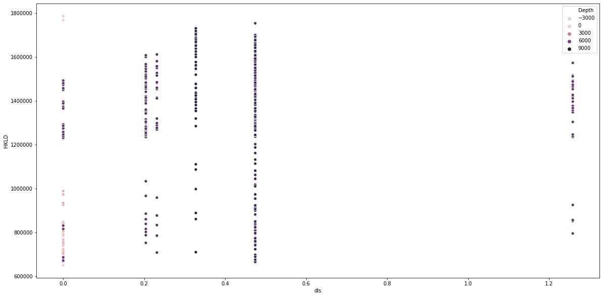
Fortunately, the DLS over the course of this interval was very low, and therefore the relationship between DLS and Hookload or tight spots doesn't exist. These transformations in order to combine multiple sources of information will be especially helpful when looking at multiple wells and trying to understand relationships/etc. We will continue the EDA sections in the next week as well. We chose to use forward fill, vs interopolate for DLS, BR and TR since it's difficult to say how the DLS changed over the course length between surveys (may have been drilling with a motor where most of the DLS occurred during the slide portion, etc).
To date we have looked at querying Azure Blob Storage, stacking and interpreting WITSML files together into a pandas dataframe - along with some basic transformations. In this week we analyzed the BHA and trajectory WITSML files and incorporated trajectory data into logging data.
With this stacked data, we can begin to better understand the wellbore construction process.