Exploratory Data Analysis
Today we will take up where we left off on the last blog where we had imported log data into a pandas dataframe for a particular well. From this data we will now explore the dataset via quick EDA and visualizations.
# Import required libraries & packages
from azure.storage.blob import BlockBlobService
import pandas as pd
import xml.etree.ElementTree as ET
from bs4 import BeautifulSoup
from collections import defaultdict
import seaborn as sns
import numpy as np
import matplotlib.pyplot as plt
%matplotlib inline
# List the account name and sas_token *** I have removed the SAS token in order to allow the user to register properly thorugh Equinor's data portal
azure_storage_account_name = 'dataplatformblvolve'
sas_token = 'sv=2018-03-28&sr=c&sig=cEL7YkHB5tZoUAr2m4teRmLohaARUHWjaVYpLxqUHzs%3D&se=2020-03-03T16%3A22%3A51Z&sp=rl'

# Create a service and use the SAS
sas_blob_service = BlockBlobService(
    account_name=azure_storage_account_name,
    sas_token=sas_token,
)

filename = 'WITSML Realtime drilling data/Norway-StatoilHydro-15_$47$_9-F-14/1/log/1/1/1'

blob = sas_blob_service.list_blobs('pub', filename)
for b in blob:
    print(b.name)
WITSML Realtime drilling data/Norway-StatoilHydro-15_$47$_9-F-14/1/log/1/1/1/00001.xml
WITSML Realtime drilling data/Norway-StatoilHydro-15_$47$_9-F-14/1/log/1/1/1/00002.xml
WITSML Realtime drilling data/Norway-StatoilHydro-15_$47$_9-F-14/1/log/1/1/1/00003.xml
def units(df):
    '''
    The intent of this function is to convert units from metric to US

    Input: df - pandas dataframe
    Output: df - pandas dataframe with columns transformed based on current units

    '''
    corr_columns = []
    for col in df.columns:
        corr_columns.append(col.split(' - ')[0])
        try:
            df[col] = df[col].astype(float)
        except:
            continue
        # Analyze column units and transform if appropriate
        # Future work will use dictionary rather than series of if statements
        if (col.split(' - ')[1] == 'm') | (col.split(' - ')[1] == 'm/h') | (col.split(' - ')[1] == 'm/s2'):
            df[col] = df[col].astype(float) * 3.28084
        if col.split(' - ')[1] == 'degC':
            df[col] = (df[col].astype(float) * 9/5) + 32
        if col.split(' - ')[1] == 'm3':
            df[col] = df[col].astype(float) * 6.289814
        if col.split(' - ')[1] == 'kkgf':
            df[col] = df[col].astype(float) * 2.2
        if col.split(' - ')[1] == 'kPa':
            df[col] = df[col].astype(float) * 0.145038
        if col.split(' - ')[1] == 'L/min':
            df[col] = df[col].astype(float) * 0.264172875
        if col.split(' - ')[1] == 'g/cm3':
            df[col] = df[col].astype(float) * 8.3454
        if col.split(' - ')[1] == 'kN.m':
            df[col] = df[col].astype(float) * 0.737562

    df.columns = corr_columns
    return df
filename = 'WITSML Realtime drilling data/Norway-StatoilHydro-15_$47$_9-F-14/1/log/1/1/1'
blob = sas_blob_service.list_blobs('pub', filename)
master_df = pd.DataFrame()
for x, file in enumerate(blob):
    blob = sas_blob_service.get_blob_to_text('pub', file.name)
    soup = BeautifulSoup(blob.content, 'xml')
    log_names = soup.find_all('mnemonicList')
    unit_names = soup.find_all('unitList')
    header = [i + ' - ' + j for i, j in zip(log_names[0].string.split(","), unit_names[0].string.split(","))]
    data = soup.find_all('data')
    df = pd.DataFrame(columns=header,
                      data=[row.string.split(',') for row in data])
    df = df.replace('', np.NaN)
    df = units(df)
    if x == 0:
        master_df = df
    else:
        master_df = pd.concat([master_df, df], sort = False)
print('Total Length of DataFrame: ' + str(len(master_df)))
master_df.head()
Total Length of DataFrame: 30000
| DEPTH | G_IC5 | BDDI | INCL_CONT_RT | TDH | TVA | SHKRSK_RT | G_NC5 | MFOP | NRPM_RT | ... | AJAM_MWD | SHKPK_RT | STICK_RT | G_C3 | ECD_MWD | G_IC4 | DRILLTM_RT | G_C1 | G_NC4 | CRS1 | |
|---|---|---|---|---|---|---|---|---|---|---|---|---|---|---|---|---|---|---|---|---|---|
| 0 | 0.000000 | NaN | NaN | NaN | NaN | NaN | NaN | NaN | NaN | NaN | ... | NaN | NaN | NaN | NaN | NaN | NaN | 601.201 | NaN | NaN | NaN |
| 1 | 300.688986 | NaN | NaN | NaN | NaN | NaN | NaN | NaN | NaN | NaN | ... | NaN | NaN | NaN | NaN | NaN | NaN | NaN | NaN | NaN | NaN |
| 2 | 301.299222 | NaN | NaN | NaN | NaN | NaN | NaN | NaN | NaN | NaN | ... | NaN | NaN | NaN | NaN | NaN | NaN | NaN | NaN | NaN | NaN |
| 3 | 301.610902 | NaN | NaN | NaN | NaN | NaN | NaN | NaN | NaN | NaN | ... | NaN | NaN | NaN | NaN | NaN | NaN | NaN | NaN | NaN | NaN |
| 4 | 302.240823 | NaN | NaN | NaN | NaN | NaN | NaN | NaN | NaN | NaN | ... | NaN | NaN | NaN | NaN | NaN | NaN | NaN | NaN | NaN | NaN |
5 rows × 58 columns
A quick walkthrough of the code that we just ran through - to re-familiarize ourselves with last weeks work. We connected to the blob service hosted on Azure storage. Then using that connection we download three different xml (WITSML) log files located under the directory: WITSML Realtime drilling data/Norway-StatoilHydro-15_$47$9-F-14/1/log/1/1/1. This folder structure tells us that we are in the Norway-StatoilHydro-15$47$_9-F-14 well and grabbing a series of log files. We then loop through the three log files, read in the data and append them to the maser_df pandas dataframe.
In last weeks blog we looked at the data structure / missing data / etc of one of these three files. Now that we have a 'completed' log we can do a similar analysis:
plt.figure(figsize = (15,5))
plt.bar(range(len(master_df.isna().sum())), list(master_df.isna().sum().values / len(master_df)), align='center')
plt.xticks(range(len(master_df.isna().sum())), master_df.columns.to_list(), rotation='vertical')
plt.title('Proportion NA Data by Column')
plt.show()
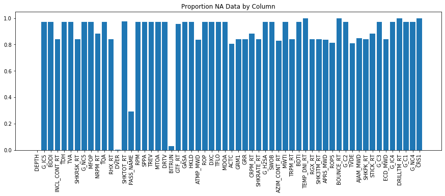
Unfortunately - similar to the previous analysis - most channels contain missing data. Similar to last weeks analysis - we can leave it like this, we could see if there are any other data sources, we could see if there is time based data that can be re-indexed to depth based and determine if there is less missing data. This latter approach does have a few asterics: - The dataset should be filtered to only include 'on-bottom' data. This can be achieved by subtracting bit depth from hole depth and only selecting data where the result of that subtraction is <0.5ft (good to have a little buffer). - Some data may not be appropriate to write to bit depth (for example MWD gamma ray is located back at the MWD tool, which may be 20-100ft behind the bit). In this case - it will be pertinent to read in the BHA file for that particular run, look for the sensor offsets and use this information to subtract depth from the bit depth to correctly write the sensor depth to a depth based file.
Our other option is to use interpolation like we did in the previous weeks example. Since we've already covered interpolation last week - we will look at transforming a time based dataset into depth based. Located under the folder WITSML Realtime drilling data/Norway-StatoilHydro-15_$47$_9-F-14/1/log/2 are time based log files. We will import the time based data similar to the depth based and save it to a master dataframe file:
filename = 'WITSML Realtime drilling data/Norway-StatoilHydro-15_$47$_9-F-14/1/log/2/1/1'
blob = sas_blob_service.list_blobs('pub', filename)
master_df = pd.DataFrame()
for x, file in enumerate(blob):
    blob = sas_blob_service.get_blob_to_text('pub', file.name)
    soup = BeautifulSoup(blob.content, 'xml')
    log_names = soup.find_all('mnemonicList')
    unit_names = soup.find_all('unitList')
    header = [i + ' - ' + j for i, j in zip(log_names[0].string.split(","), unit_names[0].string.split(","))]
    data = soup.find_all('data')
    df = pd.DataFrame(columns=header,
                      data=[row.string.split(',') for row in data])
    df = df.replace('', np.NaN)
    df = units(df)
    if x == 0:
        master_df = df
    else:
        master_df = pd.concat([master_df, df], sort = False)
print('Total Length of DataFrame: ' + str(len(master_df)))
master_df.head()
Total Length of DataFrame: 309431
| TIME | TVT | CFIA | GRR | TDH | TVDE | DCHM | STIS | TQA | ROP | ... | SPM3 | BITRUN | PD_GRAV_BHC | PDINCL | TV04 | TV06 | DVER | SWOB | MDOA | SDEP_CONT_RT | |
|---|---|---|---|---|---|---|---|---|---|---|---|---|---|---|---|---|---|---|---|---|---|
| 0 | 2008-05-09T14:57:41.040Z | 4549.611268 | 0.0 | NaN | 64.274001 | NaN | NaN | NaN | 0.014751 | 348.687671 | ... | 0.0 | NaN | NaN | NaN | 472.365021 | 324.743103 | 3551.574981 | 0.0 | 5.42451 | NaN |
| 1 | 2008-05-09T14:57:45.014Z | 4546.277483 | 0.0 | NaN | 64.274001 | NaN | 3553.215401 | NaN | 0.014751 | 348.687671 | ... | 0.0 | NaN | NaN | NaN | 472.365021 | 324.805991 | 3551.574981 | 0.0 | 5.42451 | NaN |
| 2 | 2008-05-09T14:57:50.026Z | 4543.761787 | 0.0 | NaN | 64.274001 | NaN | NaN | NaN | 0.014751 | 348.687671 | ... | 0.0 | NaN | NaN | NaN | 472.553709 | 324.805991 | 3551.574981 | 0.0 | 5.42451 | NaN |
| 3 | 2008-05-09T14:57:54.000Z | 4542.000455 | 0.0 | NaN | 64.274001 | NaN | NaN | NaN | 0.014751 | 348.687671 | ... | 0.0 | NaN | NaN | NaN | 472.553709 | 324.805991 | 3551.574981 | 0.0 | 5.42451 | NaN |
| 4 | 2008-05-09T14:57:59.011Z | 4540.490961 | 0.0 | NaN | 64.274001 | NaN | NaN | NaN | 0.014751 | 348.687671 | ... | 0.0 | NaN | NaN | NaN | 472.553709 | 324.805991 | 3551.574981 | 0.0 | 5.42451 | NaN |
5 rows × 97 columns
Here we can see that time is the index of the dataset (note when we imported the dataset - we didn't specify an index so pandas wrote an integer index). We could specify the index either when defining the dataset, or after. Below we will filter the dataset for only on bottom data and then will specify the index as the depth cahnnel.
master_df = master_df[master_df['DMEA'] - master_df['DBTM'] < 1]
master_df['DMEA'] = master_df['DMEA'].round(2)
depth_df = master_df.groupby(['DMEA']).mean()
depth_df.head()
| TVT | CFIA | GRR | TDH | TVDE | DCHM | STIS | TQA | ROP | SHKRSK_RT | ... | SPM3 | BITRUN | PD_GRAV_BHC | PDINCL | TV04 | TV06 | DVER | SWOB | MDOA | SDEP_CONT_RT | |
|---|---|---|---|---|---|---|---|---|---|---|---|---|---|---|---|---|---|---|---|---|---|
| DMEA | |||||||||||||||||||||
| 3443.01 | 4811.393296 | 0.0 | NaN | 63.644000 | NaN | 3443.012097 | NaN | 2.979750 | 348.687671 | NaN | ... | 69.0 | NaN | NaN | NaN | 470.635338 | 322.541667 | 3441.371677 | 4.767173 | 5.42451 | NaN |
| 3443.04 | 4792.523701 | 0.0 | NaN | 63.635000 | NaN | 3443.044537 | NaN | 3.593402 | 348.687671 | NaN | ... | 69.0 | NaN | NaN | NaN | 470.610173 | 322.566824 | 3441.371677 | 5.209118 | 5.42451 | NaN |
| 3443.08 | 4768.009358 | 0.0 | NaN | 63.625999 | NaN | 3443.077378 | NaN | 3.033224 | 348.687671 | NaN | ... | 69.0 | NaN | NaN | NaN | 470.540982 | 322.730365 | 3441.371677 | 5.810343 | 5.42451 | NaN |
| 3443.11 | 4744.582833 | 0.0 | NaN | 63.625999 | NaN | NaN | NaN | 3.291001 | 348.687671 | NaN | ... | 69.0 | NaN | NaN | NaN | 470.264226 | 322.529087 | 3441.371677 | 6.348753 | 5.42451 | NaN |
| 3443.14 | 4729.405548 | 0.0 | NaN | 63.612499 | NaN | 3443.143059 | NaN | 3.186268 | 348.687671 | NaN | ... | 69.0 | NaN | NaN | NaN | 470.415207 | 322.698909 | 3441.371677 | 6.971290 | 5.42451 | NaN |
5 rows × 94 columns
Above we first filtered to remove off bottom data, then rounded the hole depth channel to the nearest hundreth of a foot, then used groupby and mean to transform the index. There is also a set_index() functionality to pandas. This will transform the data to have a depth index, but will not merge the data at the same hole depth. If you have 10 datapoints that all correspond to 100.01 ft (100.005, 100.0011..) then you will continue to have all data - which may or may not be a preferred functionality. Above we used groupby and mean to average the data. This data has now been converted to depth - but as previously mentioned our sensor data that isn't written to bit depth needs to be updated - this can be difficult, there are a few ways to accomplish this: - If the index (hole depth) contains evenly spaced rows we can shift the data using .shift() at the end of the column - The data above isn't evenly spaced which makes it more complicated - the way to accomodate sensor data would be accomplished by separating the column into a new dataframe, drop it from the original dataframe then merge the two back together, below we will show how this can be accomplished for the PD_GRAV_BHC channel:
df_pd = depth_df['PD_GRAV_BHC']
df_pd = df_pd.reset_index()
df_pd['DMEA'] = df_pd['DMEA'] - 8.5
df_pd = df_pd.set_index('DMEA')
df_pd.head()
| PD_GRAV_BHC | |
|---|---|
| DMEA | |
| 3434.51 | NaN |
| 3434.54 | NaN |
| 3434.58 | NaN |
| 3434.61 | NaN |
| 3434.64 | NaN |
depth_df = depth_df.drop(['PD_GRAV_BHC'], axis = 1)
depth_df = pd.concat([depth_df, df_pd], axis = 1, sort = False)
depth_df.head()
| TVT | CFIA | GRR | TDH | TVDE | DCHM | STIS | TQA | ROP | SHKRSK_RT | ... | SPM3 | BITRUN | PDINCL | TV04 | TV06 | DVER | SWOB | MDOA | SDEP_CONT_RT | PD_GRAV_BHC | |
|---|---|---|---|---|---|---|---|---|---|---|---|---|---|---|---|---|---|---|---|---|---|
| DMEA | |||||||||||||||||||||
| 3434.51 | NaN | NaN | NaN | NaN | NaN | NaN | NaN | NaN | NaN | NaN | ... | NaN | NaN | NaN | NaN | NaN | NaN | NaN | NaN | NaN | NaN |
| 3434.54 | NaN | NaN | NaN | NaN | NaN | NaN | NaN | NaN | NaN | NaN | ... | NaN | NaN | NaN | NaN | NaN | NaN | NaN | NaN | NaN | NaN |
| 3434.58 | NaN | NaN | NaN | NaN | NaN | NaN | NaN | NaN | NaN | NaN | ... | NaN | NaN | NaN | NaN | NaN | NaN | NaN | NaN | NaN | NaN |
| 3434.61 | NaN | NaN | NaN | NaN | NaN | NaN | NaN | NaN | NaN | NaN | ... | NaN | NaN | NaN | NaN | NaN | NaN | NaN | NaN | NaN | NaN |
| 3434.64 | NaN | NaN | NaN | NaN | NaN | NaN | NaN | NaN | NaN | NaN | ... | NaN | NaN | NaN | NaN | NaN | NaN | NaN | NaN | NaN | NaN |
5 rows × 94 columns
In the first cell we separate out the PD Grav variable, reset the index so that DMEA is its own column, then subtract the sensor offset distance from the BHA file. We then reset the index so that we can use the concat function.
In the second column, we drop the PD Grav variable from the original depth dataset, then use concat to combine the two with the sensor adjusted depth.
We can now visualize to see if our time to depth conversion helped improve NA values:
plt.figure(figsize = (15,5))
plt.bar(range(len(depth_df.isna().sum())), list(depth_df.isna().sum().values / len(depth_df)), align='center')
plt.xticks(range(len(depth_df.isna().sum())), depth_df.columns.to_list(), rotation='vertical')
plt.title('Proportion NA Data by Column')
plt.show()
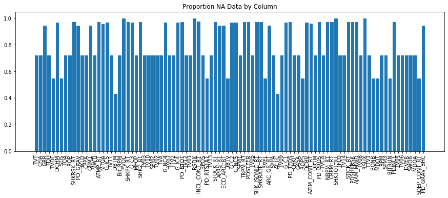
What we can see is that we have more channels compared to the original depth dataset - and the proportion of missing data, while still large, is significantly reduced compared to the depth dataset. If we set the depth sample rate to the nearest 0.5 ft we will likely improve missing proprotion values as well:
depth_df = depth_df.reset_index()
depth_df['DMEA'] = round(depth_df['DMEA'] * 2) / 2
depth_df = depth_df.groupby('DMEA').mean()
depth_df.head()
| TVT | CFIA | GRR | TDH | TVDE | DCHM | STIS | TQA | ROP | SHKRSK_RT | ... | SPM3 | BITRUN | PDINCL | TV04 | TV06 | DVER | SWOB | MDOA | SDEP_CONT_RT | PD_GRAV_BHC | |
|---|---|---|---|---|---|---|---|---|---|---|---|---|---|---|---|---|---|---|---|---|---|
| DMEA | |||||||||||||||||||||
| 3434.5 | NaN | NaN | NaN | NaN | NaN | NaN | NaN | NaN | NaN | NaN | ... | NaN | NaN | NaN | NaN | NaN | NaN | NaN | NaN | NaN | NaN |
| 3435.0 | NaN | NaN | NaN | NaN | NaN | NaN | NaN | NaN | NaN | NaN | ... | NaN | NaN | NaN | NaN | NaN | NaN | NaN | NaN | NaN | NaN |
| 3435.5 | NaN | NaN | NaN | NaN | NaN | NaN | NaN | NaN | NaN | NaN | ... | NaN | NaN | NaN | NaN | NaN | NaN | NaN | NaN | NaN | NaN |
| 3436.0 | NaN | NaN | NaN | NaN | NaN | NaN | NaN | NaN | NaN | NaN | ... | NaN | NaN | NaN | NaN | NaN | NaN | NaN | NaN | NaN | NaN |
| 3436.5 | NaN | NaN | NaN | NaN | NaN | NaN | NaN | NaN | NaN | NaN | ... | NaN | NaN | NaN | NaN | NaN | NaN | NaN | NaN | NaN | 444.959 |
5 rows × 94 columns
plt.figure(figsize = (15,5))
plt.bar(range(len(depth_df.isna().sum())), list(depth_df.isna().sum().values / len(depth_df)), align='center')
plt.xticks(range(len(depth_df.isna().sum())), depth_df.columns.to_list(), rotation='vertical')
plt.title('Proportion NA Data by Column')
plt.show()
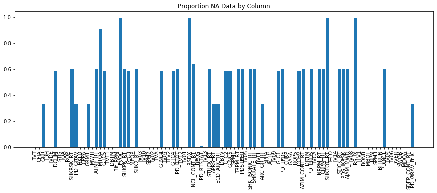
We can see that we have now substantially reduced the missing values in our dataset - which is very good. It may be questioned whether averaging to the nearest foot is appropriate - this would be dictated by the dataset. In general many channels will have a resolution at or greater than 0.5 ft, along with depth uncertainty, it can be argued that averaging to the nearest half foot is OK. If running wireline logs such as a resistivity image log, averaging to the nearest half foot may destroy some of the tiny fracture features contained within the log and would not be appropriate.
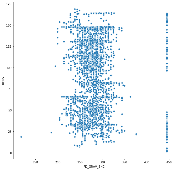
With this data it is very possible to inspect relationships in our data:
import seaborn as sns
plt.figure(figsize = (10,10))
sns.scatterplot('PD_GRAV_BHC', 'ROP5', data = depth_df)
<matplotlib.axes._subplots.AxesSubplot at 0x193ee58b860>
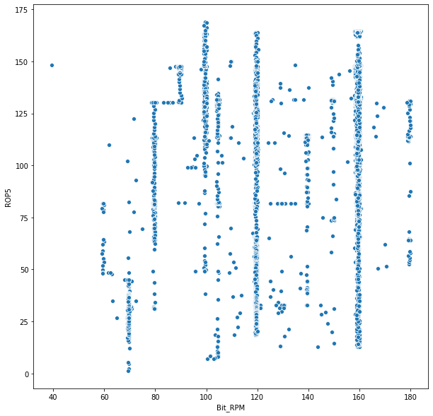
import seaborn as sns
plt.figure(figsize = (10,10))
sns.scatterplot('Bit_RPM', 'ROP5', data = depth_df)
<matplotlib.axes._subplots.AxesSubplot at 0x193803bb6d8>
Further EDA can also be carried out using standard Python EDA plots and analysis. The primary point stressed in this dataset is the importance of understanding the data. This is often the most laborious and painful part of analysis, often constituting excessive amount of time - but is also the most crucial. ML algorithms often struggle with missing data - understanding how to handle missing data most appropriately and accurately is essential to deriving insightful meaning from an ML model and/or business intelligence.
We saw that time based data transformed into depth based may provide a more complete dataset, and we saw how to accurately complete this process. In oil and gas data missing / incorrect data is very commonplace and should be expected. Taking the time to understand the dataset, understand its limitations and develop ways to improve the data contained is essential. Doing so sets the ability to then accurately use the data and derive meaning from it.
This EDA is by no means complete - many channels after converting time to depth still need to be sensor corrected. It is also pertinent to remove outlier data: - In the plot of PD gamma vs ROP we see a straight line near 440 API. Most likely this is some kind of default value as it's generally an outlier in the gamma dataset - but occurs frequently. Having more domain knowledge to understand this is important - Many times when setting or pulling slips hookload can increase/decrease abruptly causing a spike in the data. Especially when converting from time to depth based - these spikes which don't reflect the drilling process need to be removed. In others - such as detecting overpull and potential tight hole - these spikes can be quintessential.
Understanding the domain of the problem you're trying to solve, and the acceptable EDA to solve that problem are essential. This serves as a brief priner into the EDA analysis of an oil and gas dataset.